A GDP density map of the world

GDP is the value of everything a place produces in a year; density is that value divided by the land it sits on, here in dollars per square kilometre. A quarter of the world’s GDP comes from 0.15% of its land, a few hundred places such as Manhattan, the City of London and the Pearl River Delta, while the interior of Chad or the Alaskan bush produce about a thousand dollars per km². That is seven orders of magnitude, and I wanted to see it on one map.

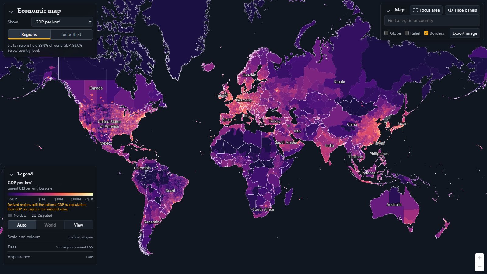
What the map shows

Every shape is a region for which an official statistic of GDP exists: 6,513 of them hold 99.8% of world GDP, and 93.6% sit below country level. Country maps of GDP hide almost everything (Germany is one colour, although the Ruhr and the Mecklenburg lake district have little in common), so each country is drawn at the finest level it publishes: US counties, European NUTS3 districts, Chinese prefectures, Brazilian immediate regions, Indian and Japanese states. Clicking a region gives its value, its population and area, and where each number comes from and how it was derived.

The colour is GDP per km² of the region’s area. It is a measure of how much economy is packed onto the land, not of how rich anyone is: a megacity of 20 million people and a refinery town can be equally dense. Three rules decided what goes in:

1. Only sourced numbers. Statistics offices, or aggregators that republish them (Eurostat, the OECD); Wikipedia as a flagged fallback where its tables cite an office. No night-light or machine-learning grids: a map built on a model shows the model.
2. The finest level each country publishes. States if it publishes states, counties if counties, otherwise one region.
3. Regions add up to the country. A region’s value is its share of the national total times the World Bank’s GDP for the reference year, so currencies and years are comparable and the map never shows more economy than exists.

The same data gives other indicators, switched under Show: GDP per capita (the usual measure of wealth, which reorders the map: dense but poor districts drop, sparse oil and mining regions rise), population density, and the totals GDP and population. The legend can also convert to constant dollars of a base year, and Estimates hides values that come from a model or a population split rather than a statistic.

Sources: a patchwork, shown on North America

There is no global table of regional GDP. The map rests on 47 sources, and each country publishes at a different level, in different years and codes. North America shows the three typical cases in one view.

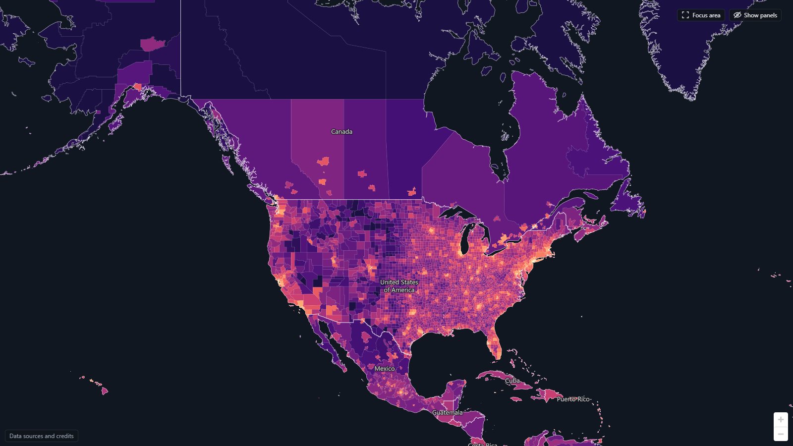
• United States: very detailed. The Bureau of Economic Analysis publishes GDP for all 3,100 counties, and the Census population. This is the best case, with the opposite problem: a county in Nevada is as large as a European country, and gets one colour for a casino town and a desert.
• Canada: huge lands of nothing. Statistics Canada publishes provinces and 42 metropolitan areas, nothing in between. Each province is therefore its metro areas plus a “rest of province”, and the rests are enormous: Nunavut, the Northwest Territories and northern Quebec are millions of km² in one near-black colour, with Toronto or Calgary as a small dot. That is honest, but it looks like another planet next to the counties directly south.
• Mexico: too detailed, too small. Mexico publishes GDP only per state. The economic census has value added for each of roughly 2,500 municipalities, which is too many and too small to read. So the municipalities are consolidated into 92 metropolitan areas plus the rest of each state, and each state’s GDP is split between them by census value added. That is a model, and the map flags it as derived.

Elsewhere it is the same in other forms: Brazil’s 5,570 municipalities are grouped into 509 immediate regions; China’s prefecture GDP comes from a Wikipedia list citing the provincial yearbooks; Russia comes through Wikipedia because Rosstat’s site could not be reached without turning off certificate checks; and for 20 large countries with no regional GDP at all (Algeria, Ethiopia, Saudi Arabia and others) the national GDP is split by population into at most three density zones, marked as derived. A crosswalk matches each source’s codes to shapes, and a pipeline checks that regions cover the country without overlap and sum to its national total.

Smoothing: dense and empty, ignoring borders

Regions are still administrative units: a rich city and its poor hinterland get one colour if they share a district, and a border cuts an economic area in two. The smoothed layer asks instead: how much GDP is within reach of a point, per km² of land within reach? GDP and land are spread over a 5 to 10 km grid, both blurred with the same distance kernel (radius 15 to 150 km), and one is divided by the other. Land, not area, is the denominator, so a coastal city is not diluted by the sea next to it. The surfaces are computed in the pipeline and shipped as lossless WebP images with a 16-bit logarithmic code in the colour channels, which the browser decodes on the GPU.

Smoothing is shown in six colour classes, so the economic regions read as areas rather than gradients.

Europe

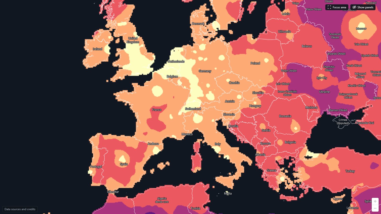
• The yellow banana: the densest class forms a continuous arc from the English Midlands and London through Benelux and the Rhine valley down to Switzerland and northern Italy. Geographers call it the Blue Banana; here it falls out of the data without anyone drawing it, and it does not stop at any frontier.
• Islands of density in an orange sea: Paris, Madrid, Barcelona, Vienna, Munich, Berlin, Warsaw, Budapest, Milan and Rome, each its own.
• The empty centre of Spain: Madrid is a single yellow dot surrounded by the least dense class of Western Europe, the Meseta of Castile, Aragón and Extremadura. Spain’s economy is its coasts and Madrid. The French Massif Central is the same case.
• The east: most of Poland is orange, the Balkans are red and Ukraine purple, and Moscow stands alone in a large, thin Russian interior.

East Asia, with the scale fitted to the view

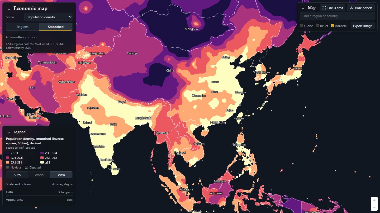
Asia is where the world scale fails: China’s coast and Japan fill the top class and everything else sinks into red and purple. Setting the legend’s scale to View fits the six classes to what is on screen. The class limits change (the legend on the image shows them: the top class starts at $4.6M per km²), so colours now compare places in this view with each other, not with the rest of the world.

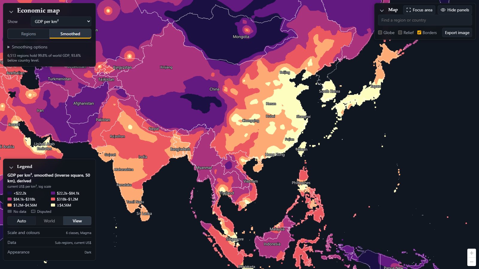
• China’s coast is a dense class that runs almost without a break from Beijing and Tianjin through the Yangtze delta around Shanghai to the Pearl River Delta with Hong Kong. Behind it the density drops fast: the Sichuan basin around Chongqing is a plateau of its own, and Tibet, Qinghai and Xinjiang are the largest empty region of the map.
• Japan is a ribbon: Tokyo, Nagoya and Osaka form the Pacific belt, with Hokkaido and the Sea of Japan coast a class below.
• India now separates: Delhi and the Ganges plain, Mumbai, and the south are orange and red fields with the Rajasthan desert and the Deccan between.
• South-East Asia: Bangkok, Singapore and Jakarta stand out, the rest is red and purple.
• Mongolia is the darkest area, with Ulaanbaatar as the only bright dot.

Two variants help reading: Local excess divides each place by its wider surroundings, showing which towns stand out from their region; Relief turns the surface into terrain, the densest places as mountains.

Population density, quickly

Switch Show to population density and the same smoothing applies to people per km². Population is where the picture of Asia is completely different: the whole Indo-Gangetic plain from Punjab to Bangladesh joins eastern China in the top class, while GDP concentrates on the Chinese coast and Japan. The gap between the two maps is productivity: India has the people but not yet the density of output.

Globe

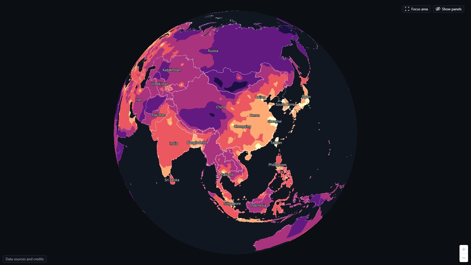
The flat map is Web Mercator, which inflates the north. Globe shows true areas and works on the smoothed layer too: from this side the Eurasian landmass shows the bright arc from Japan through the Chinese coast to India as one structure.

Focus area

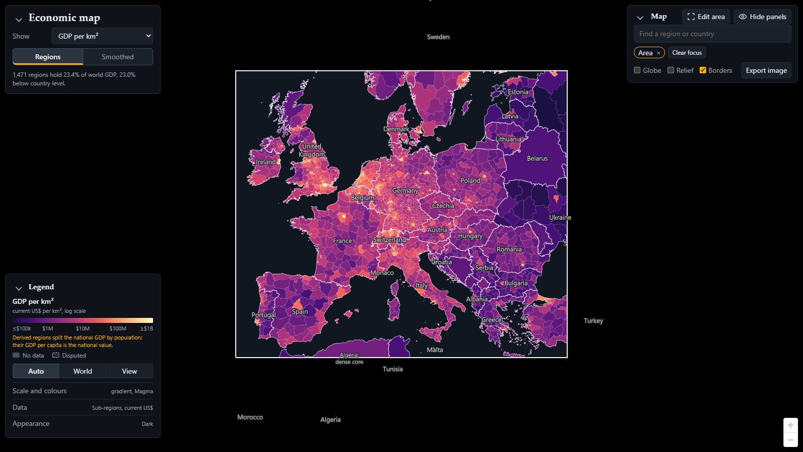
On the flat map, Focus area limits the map to regions you pick or a box you draw, and fits the colours to that selection. Here Europe at NUTS3 level in GDP per km²: with the rest of the world out of the scale, the Ruhr, the Randstad, Paris and London, and the Po valley stand clearly apart in a continent otherwise coloured evenly. Together with Export image (a PNG of the view or a drawn frame, with title, legend and credits) this is how most images here were made. Every view is also a link: the address bar holds the full state, so copying it shares exactly what you see, as the images here do.

What to keep in mind

The map shows where GDP is booked: head offices, refineries and tax-efficient addresses pull it to where the books are, and commuter cities look richer per person than the suburbs where the commuters live. Some shares are older than 2024 and some countries lack a level; the data notes list every source, licence and known gap. The smoothed surfaces carry no information finer than the regions they are made from.

I built it over ten days in October 2026 with Claude Code: I set the direction and made the decisions, agents wrote and reviewed the code, often overnight. The code and the full recipe are on GitHub under the MIT licence; the data keeps its sources’ licences.