Julia for joint models

In an oncology trial every patient produces two kinds of data: tumour-size measurements over time, and a time to an event such as death. A joint model fits both at once, so that the tumour’s trajectory informs the risk. My master’s thesis asked whether such models, with a non-linear tumour model, can be built and checked in one language, Julia, instead of R wrapped around Stan and C++. I wrote it at ETH Zürich’s Seminar for Statistics with Roche in Basel, supervised by Prof. Peter Bühlmann, and it was graded 6 out of 6.

This page is the statistical side: the hazard, the joint likelihood, and how the fitted model was checked. The software side is in the post on JointSurvivalModels.jl, the package that came out of it.

The hazard

Let $T \ge 0$ be the time to the event, with distribution function $F$, density $f$ and survival function $S(t) = P(T > t)$. The hazard is the rate at which the event happens at time $t$, given that it has not happened before:

$$h(t) = \lim_{\Delta \to 0^+} \frac{P(t \le T < t + \Delta \mid T \ge t)}{\Delta} = \frac{f(t)}{S(t)}.$$

It is a rate, not a probability: it has units of one over time and can exceed 1. Among the patients still at risk at time $t$, about $h(t)\,\Delta$ of them have the event in the next short interval $\Delta$.

Since $f = -S'$, the hazard is $h = -\tfrac{d}{dt}\log S$. Integrating gives the cumulative hazard $H$ and, from it, everything else:

$$H(t) = \int_0^t h(u)\,du, \qquad S(t) = e^{-H(t)}, \qquad f(t) = h(t)\,e^{-H(t)}.$$

So the hazard alone defines the distribution. Any non-negative function whose integral diverges is the hazard of exactly one distribution on $[0, \infty)$. This is why survival models are written in terms of $h$: it is the quantity that is easy to reason about (“the risk doubles”) and easy to modify.

Censoring. A study ends, or a patient leaves it, before the event. We then observe $t = \min(T, c)$ and an indicator $\delta$, 1 for an event and 0 for a censored time. An event contributes its density to the likelihood, a censored time only the fact of survival up to $t$:

$$\mathcal{L}(t, \delta) = f(t)^{\delta}\,S(t)^{1-\delta}, \qquad \log \mathcal{L}(t, \delta) = \delta \log h(t) - H(t).$$

Covariates. Cox’s proportional-hazards model multiplies a baseline hazard by an exponential, $h(t \mid x) = h_0(t)\exp(\beta^\top x)$. The ratio of two patients’ hazards is then $\exp(\beta^\top (x_1 - x_2))$, free of $t$ and of $h_0$, which is what makes the coefficients interpretable.

The longitudinal model

Patient $i$ has measurements $y_{ij}$ at times $t_{ij}$. A mixed-effects model gives every patient the same curve $m$ with their own parameters $\psi_i$, drawn around population values: $m_i(t) = m(t, \psi_i)$. With an error model on top, each measurement has a density $p_i(y_{ij} \mid t_{ij})$.

Nothing here requires $m$ to be linear, and in oncology it is not. Following Kerioui et al. (2020), the sum of the longest tumour diameters grows exponentially until treatment starts at $t_x$; after that a fraction $\varphi$ of the tumour shrinks at rate $d$ while the rest keeps growing at rate $g$:

$$\text{SLD}(t, \psi) = \begin{cases} \text{BSLD}\, e^{g t} & t < t_x \\ \text{BSLD}\, e^{g t_x}\big(\varphi\, e^{-d (t - t_x)} + (1 - \varphi)\, e^{g (t - t_x)}\big) & t \ge t_x \end{cases}$$

with $\psi = (\text{BSLD}, g, d, \varphi)$ per patient: log-normal random effects on the first three, a logit-normal one on $\varphi$, and a multiplicative error $y_{ij} = \text{SLD}(t_{ij}, \psi_i)(1 + e_{ij})$.

Joining them

A joint model puts the patient’s curve into their hazard, in the same place Cox puts a covariate:

$$h_i(t) = h_0(t)\,\exp\big(\gamma \cdot L(m_i(t))\big).$$

The link $L$ says which feature of the curve drives the risk. It acts on the curve, not on a number: the current tumour size $m_i(t)$, its growth rate $\tfrac{d}{dt} m_i(t)$, or a summary of the whole trajectory such as the time at which the tumour starts to grow again. The coefficient $\gamma$ is the quantity of interest: how strongly does the tumour’s course move the risk of death?

Given the parameters $\theta$, which include every $\psi_i$, the two kinds of data are independent, and the log-likelihood is a sum of a survival part and a longitudinal part:

$$\ell(\theta) = \sum_i \big[\delta_i \log h_i(t_i) - H_i(t_i)\big] + \sum_{i,j} \log p_i(y_{ij} \mid t_{ij}).$$

Compared with feeding the measured tumour sizes into a Cox model as a time-varying covariate, this uses a smooth curve at every $t$ instead of noisy values at visit times, and it carries the uncertainty about that curve into $\gamma$.

Two caveats belong here. The longitudinal part treats a patient’s measurements as independent given $\psi_i$, which is a strong assumption for a tumour that either grows or shrinks. And the exponential form is a convention inherited from Cox; other ways of letting $m_i$ act on the hazard are possible.

Why this needed new software

With the SLD curve inside the exponential, $H_i(t) = \int_0^t h_i(u)\,du$ has no closed form. The established R packages (JM, JMbayes) avoid the integral by allowing only longitudinal models that are linear in their parameters. Roche’s newer package jmpost supports non-linear models, but as R wrapped around Stan and C++, and at the time with a fixed menu of models.

In the thesis the integral is computed numerically (adaptive Gauss–Kronrod quadrature), and the model is fitted by Bayesian inference: priors on $\theta$, and the NUTS sampler of Turing.jl on the log-likelihood above. The decisive step was to stop adding the survival term to the log-likelihood by hand and instead hand the sampler a proper probability distribution, defined by nothing but its hazard. Two things a statistician needs depend on that:

• leave-one-out cross-validation (PSIS-LOO) needs to know which observation produced which likelihood term;
• posterior predictive checks need to simulate event times, here by inverse transform sampling from $F = 1 - e^{-H}$.

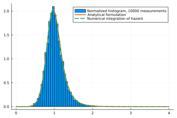
As a check of the numerics, a log-logistic distribution defined only through its hazard reproduces the analytical density, and 10,000 simulated event times fall on the same curve:

How that distribution is built, and what it became, is the subject of the package post.

Does it get the right answer?

Kerioui et al. published a simulated data set (100 patients, 655 tumour measurements) together with their R/Stan code. I fitted the same model with the same priors and the same sampler settings (NUTS, 200 warm-up and 400 posterior draws) in both, and compared the posterior means:

Parameter	True value	R/Stan (original)	Julia/Turing (mine)
Baseline tumour size $\mu_{\text{BSLD}}$	60	62.3	61.2
Growth rate $\mu_g$	0.0015	0.0018	0.0018
Treated fraction $\mu_\varphi$	0.2	0.20	0.18
Baseline scale $\lambda$	1450	1505	1512
Link coefficient $\gamma$	0.01	0.0103	0.0104

The two implementations agree with each other and with the truth. Where both miss, on one random-effect variance, both also flag it with a high $\hat R$. The chains are short, so this shows agreement between two implementations, not a converged analysis.

Checking a fitted model

A model you cannot check is not finished. The thesis builds the checks into the same workflow:

• Posterior predictive checks for the trajectories: per patient, the 95% band of simulated measurements against the observed ones.
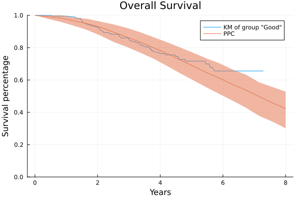
• Posterior predictive checks for survival: simulated event times are hard to compare one by one, so each simulated data set is reduced to its Kaplan–Meier curve, and the observed Kaplan–Meier curve should lie inside the band of the simulated ones.
• Residuals: the Cox–Snell residual of patient $i$ is $r_i = H_i(t_i)$. If the model is right, the pairs $(r_i, \delta_i)$ look like a censored sample from a unit exponential. The martingale residual $\delta_i - r_i$ is observed minus expected events and shows which patients, or which covariate values, the model fits badly.

Predicting for one patient

The plot that uses everything at once is the prediction for a single patient. Patient 25 was still alive at their last visit, around day 700 (the vertical line), so their survival time is censored there. The question is what the fitted model says about this patient from that day on.

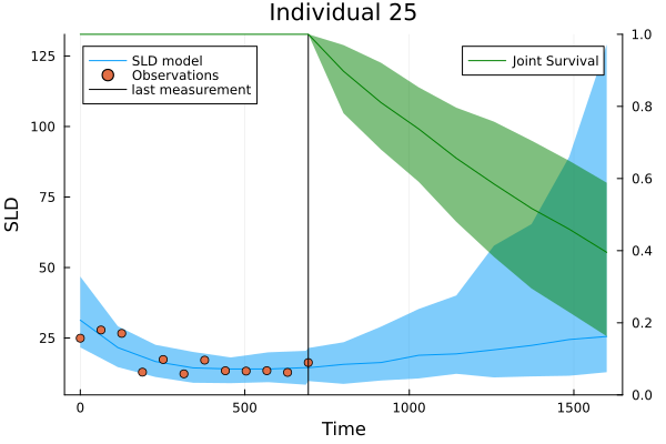
Both bands come from the same posterior draws $\theta^{(1)}, \dots, \theta^{(S)}$. Each draw contains this patient’s own curve parameters $\psi_i^{(s)}$, and their posterior has already learned from both kinds of data: the measurements, and the fact that the patient survived to the last visit.

The tumour band (blue) is a posterior predictive interval. For every draw and every time $t$ on a grid, a new measurement is simulated from the error model around that draw’s curve,

$$\tilde y^{(s)}(t) \sim p\big(y \mid m(t, \psi_i^{(s)}), \sigma^{(s)}\big),$$

and the band is the 2.5% to 97.5% range of these simulations at each $t$. It therefore answers “where would a measurement fall?”, and it contains both the uncertainty about the curve and the measurement error. That is why the observed points should lie inside it, and mostly do. Right of the vertical line there are no measurements; the band widens because the draws disagree about how fast the tumour regrows.

The survival band (green) is a different kind of object. The quantity is the patient’s survival curve from the last visit $t^*$ on, given that they were alive then:

$$S_i(t \mid T > t^*, \theta) = \frac{S_i(t \mid \theta)}{S_i(t^* \mid \theta)} = \exp\big(-(H_i(t) - H_i(t^*))\big), \qquad t \ge t^*.$$

For a fixed $\theta$ this is one curve. It is estimated by simulation: for each posterior draw, 100 event times are drawn from the patient’s joint distribution, those before $t^*$ are discarded (which is the conditioning), and the Kaplan–Meier estimator of the rest is that draw’s curve. With no censoring in simulated data, Kaplan–Meier is just the empirical survival function. The line is the median of these curves at each $t$, and the band their 2.5% to 97.5% range.

So the green band is not an interval for when the patient dies. It is a credible band for a probability: “the chance of being alive at day 1500, given alive at day 700, is around 45%, and the data leave it between roughly 25% and 65%”. Its width has two sources: the posterior uncertainty about $\theta$, and the Monte Carlo noise of estimating each curve from at most 100 simulated times.

The two halves are linked, which is the point of a joint model. The hazard is $h_0(t)\exp(\gamma\, m_i(t))$ with $\gamma > 0$, so a draw in which the tumour regrows quickly is also a draw in which survival falls quickly.

The detour through simulation, instead of evaluating $H_i$ directly, is deliberate: the plot uses nothing but simulated data, so it works unchanged for any baseline hazard, link or tumour model.

The residuals above need each patient’s cumulative hazard from every posterior draw. To record it during sampling I first wrote a small helper distribution that always returns one value. Then I noticed that this is the Dirac distribution, which Distributions.jl already has, and used that.

What I concluded

Julia is well suited to this work. The model code stays close to the formulas above, and one language covers the model, the sampler and the diagnostics. Compared with jmpost, which tells the user clearly which models exist and how to load data, my workflow asks for more code and gives more freedom: any longitudinal model, any baseline hazard, any link. The caveat is age. The ecosystem is younger than R’s or SAS’s, and I hit rough edges along the way.

What I handed over at Roche was a documentation site of workflows for survival, longitudinal and joint models, included in the thesis appendix. The hazard-defined distribution outlived the thesis as an open-source package: JointSurvivalModels.jl.