JointSurvivalModels.jl

JointSurvivalModels.jl is a Julia package that turns a hazard function into a full probability distribution: you write one function, and you get logpdf, ccdf, rand and censoring, ready for a probabilistic programming language. Its main use is joint models of survival and longitudinal data, which have no closed-form density. I wrote it during my master’s thesis with Roche; version 1.0 was released in February 2024 under Roche’s open-source organisation insightsengineering and is in Julia’s package registry:

using Pkg
Pkg.add("JointSurvivalModels")

This page is about the software: the interface and how it is computed. For the statistics behind it (the hazard, the likelihood, model checking), see the post on the thesis.

The problem, as an interface problem

A sampler such as Turing.jl’s NUTS asks two things of every observed quantity: a log-density, to score parameters, and a way to draw samples, to simulate from the fitted model. For the usual distributions both are formulas.

Survival models are specified differently, by their hazard $h(t)$: the event rate at time $t$ among those who have not had the event yet. The density follows from it, but through an integral:

$$f(t) = h(t)\,\exp\Big(-\int_0^t h(u)\,du\Big).$$

In a joint model the hazard contains a patient’s biomarker curve, for example tumour size over time, and that curve is non-linear. The integral then has no closed form. The R packages for joint models avoid it by restricting the curve to linear models. The alternative is to compute it numerically, which raises the question of where that code lives so that the sampler still sees an ordinary distribution.

One method to implement

The package answers with an abstract type. Subtype HazardBasedDistribution, implement hazard, and the rest of the Distributions.jl interface is derived:

struct LogLogistic <: HazardBasedDistribution
    α::Real
    β::Real
end

JointSurvivalModels.hazard(d::LogLogistic, t::Real) =
    (d.β / d.α) * (t / d.α)^(d.β - 1) / (1 + (t / d.α)^d.β)

What you get, and how:

Because the type is a ContinuousUnivariateDistribution, everything written against that interface works unchanged. That includes Distributions.jl’s censored, which is how a survival time whose event was never observed enters a model.

Joint models on top

JointSurvivalModel is the ready-made subtype, with the hazard

$$h(t) = h_0(t)\,\exp\big(\gamma^\top L(M(t)) + \beta^\top x\big)$$

for any baseline hazard $h_0$, any number of longitudinal models $M$ with their links $L$, and covariates $x$. All of them are plain Julia functions of time:

jm = JointSurvivalModel(t -> 0.2, 0.5, cos)   # h(t) = 0.2 · exp(0.5 · cos t)

Inside a Turing model, a patient’s censored survival time is one line. sld is the tumour-size curve and Ψ[i] are that patient’s parameters, sampled in the same model:

surv_times[i] ~ censored(JointSurvivalModel(h₀, γ, t -> sld(t, Ψ[i])), upper = censoring)

Why a distribution

My first working joint model added the survival log-likelihood by hand with @addlogprob!. It sampled correctly and still was a dead end: the framework no longer knew which observation a term belonged to, so leave-one-out cross-validation did not work, and with nothing to call rand on, neither did predict. Making the model a distribution fixed both at once. That is the whole package: about 200 lines that compose Integrals.jl, DifferentialEquations.jl and Roots.jl behind the Distributions.jl interface.

A worked case study

The repository reproduces the oncology model of Kerioui et al. (2020): a non-linear mixed-effects model of tumour size, an exponential baseline hazard and an identity link. On their simulated data of 100 patients, 2,000 NUTS draws recover the parameters the data were generated with. The link coefficient comes out at $\gamma = 0.0103 \pm 0.0012$ against a true $0.01$, with $\hat R \approx 1$ throughout.

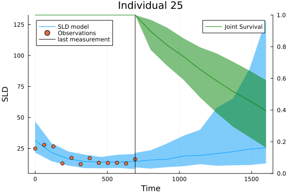
Because the distribution can also be sampled, the same fit gives individual predictions: a patient’s tumour trajectory, and their survival conditional on having survived to their last visit.

I wrote the package. Daniel Sabanés Bové, Francois Mercier and Doug Kelkhoff at Roche, my thesis supervisors there, co-authored the short software paper (the PDF above), which sets out the method and this case study. How the same model compares with the original R/Stan implementation, and how a fitted joint model is checked, is in the thesis post.